Probability

Some Basic Terms

Coin

A coin has two sides, Head and Tail. If an event consists of more than one coins, then coins are considered as. distinct, if not otherwise stated.

Die

A die has six face marked 11, 2, 3, 4, 5 and 6. If we have more than one dice, then all dice are considered as distinct, if not otherwise stated.

Playing Cards

A pack of playing cards has 52 cards. There are 4 suits (spade, heart, diamond and club) each having 13 cards. There are two colours, red (heart and diamond) and black (spade and club) each having 26 cards.

In 13 cards of each suit, there are 3 face cards namely king, queen and jack so there are in all ’12 face cards. Also, there are 16 honour cards,
4 of each suit namely ace, king, queen and jack.

Types of Experiments

1. Deterministic Experiment

Those experiments, which when repeated under identical conditions produce the same result or outcome are known as deterministic experiment,

2. Probabilistic/Random Experiment

Those experiments, which when repeated under identical conditions, do not produce the same outcome every time but the outcome in a trial is one of the several possible outcomes, called random experiment.

Important Definitions

(i) Trial Let a random experiment, be repeated under identical conditions, then the experiment is called a Trial.

(ii) Sample Space The set of all possible outcomes of an experiment is called the sample space of the experiment and it is denoted by S.

(iii) Event A subset of the sample space associated with a random experiment is called event or case.

(iv) Sample Points The outcomes of an experiment is called the sample point.

(v) Certain Event An event which must occur, whatever be the outcomes, is called a certain or sure event.

(vi) Impossible Event An event which cannot occur in a particular random experiment, is called an impossible event.

(vii) Elementary Event An event certaining only one sample point is called elementary event or indecomposable events.

(viii) Favourable Event Let S be the sample space associated with a random experiment and let E ⊂ S. Then, the elementary events belonging to E are known as the favourable event to E .

(ix)  Compound Events An event certaining more than one sample points is called compound events or decomposable events.

Probability

If there are n elementary events associated with a random experiment and m of them are favourable to an event A, then the probability of happening or occurrence of A, denoted by P(A), is given by

P(A) = m / n = Number of favourable cases / Total number of possible cases

Types of Events

(i) Equally Likely Events The given events are said to be equally likely, if none of them is expected to occur in preference to the other.

(ii) Mutually Exclusive Events A set of events is said to be mutually exclusive, if the happening of one excludes the happening of the other.

If A and B are mutually exclusive, then P(A ∩ B) = 0

(iii) Exhaustive Events A set of events is said to be exhaustive, if the performance of the experiment always results in the occurrence of atleast one of them.

If E1, E2, … , En are exhaustive events, then El ∪ E2 ∪ … ∪ E_n = S i.e., P(E₁ ∪ E₂ ∪ E₃ ∪ … ∪ E_n) = 1

(iv) Independent Events Two events A and B associated to a random experiment are independent, if the probability of occurrence or non-occurrence of A is not affected by the occurrence or non-occurrence of B.

i.e., P(A ∩ B) = P(A) P(B)

Complement of an Event

Let A be an event in a sample space S~the complement of A is the set of all sample points of the space other than the sample point in A and it is denoted by,

A’ or A = {n : n ∈ S, n ∉ A}

(i) P(A ∪ A’) = S

(ii) P(A ∩ A’) = φ

(iii) P(A’)’ = A

Partition of a Sample Space

The events A₁, A₂,…., A_n represent a partition of the sample space S, if they are pairwise disjoint, exhaustive and have non-zero probabilities. i.e.,

(i) A_i ∩ A_j = φ; i ≠ j; i,j= 1,2, …. ,n

(ii) A₁ ∪ A₂ ∪ … ∪ A_n = S

(iii) P(A_i) > 0, ∀ i = 1,2, …. ,n

Important Results on Probability

(i) If a set of events A₁, A₂,…., A_n are mutually exclusive, then

A₁ ∩ A₂ ∩ A₃ ∩ …∩ A_n = φ

P(A₁ ∪ A₂ ∪ A₃ ∪… ∪ A_n) = P(A₁) + (A₂) + … + P(A_n)

and A₁ ∩ A₂ ∩ A₃ ∩ …∩ A_n = 0

(ii) If a set of events A₁, A₂,…., A_n are exhaustive, then

P(A₁ ∪ A₂ ∪ … ∪ A_n) = 1

(iii) Probability of an impossible event is O. i.e., P(A) = 0, if A is impossible event. ,

(iv) Probability of any event in a sample space is 1. i.e., P(A) = 1

(v) Odds in favour of A = P(A) / P(A)

(v) Odds in Against of A = P(A) / P(A)

(vii) Addition Theorem of Probability

(a) For two events A and B

P(A ∪ B) = P(A) + P(B) – P(A ∩ B)

(b) For three events A, Band C

P(A ∪ B ∪ C) = P(A) + P(B) + P(C) -P(A ∩ B) – P(B ∩ C) – P(A ∩ C) + P(A ∩ B ∩ C)

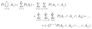
(c) For n events A₁, A₂,…., A_n

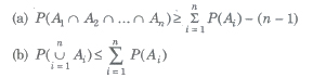
(viii) Booley’s Inequality

If A₁, A₂,…., A_n are n events associated with a random experiment, then

(ix) If A and B are two events, then

P(A ∩ B) ≤ P(A) ≤ P(A ∪ B) ≤ P(A) + P(B)

(x) If A and B are two events associated with a random experiment, then

(a) P(A ∩ B) = P(B) – P(A ∩ B)

(b) P(A ∩ B) = P(A) – P(A ∩ B)

(c)P [(A ∩ B) ∪ (A ∩ B)] = P(A) + P(B) – 2P(A ∩ B)

(d) P(A ∩ B) = 1- P(A ∪ B)

(e) P(A ∪ B) = 1- P(A ∩ B)

(f) P(A) = P(A ∩ B) + P(A ∩ B).

(g) P(B) = P(A ∩ B) + P(B ∩ A)

(xi) (a) P (exactly one of A, B occurs)

= P(A) + P(B) – 2P(A ∩ B) = P(A ∪ B) – P(A ∩ B)

(b) P(neither A nor B) = P(A’ ∩ B’) = 1 – P(A ∪ B)

(xii) If A, Band C are three events, then

(a) P(exactly one of A, B, C occurs)

= P(A) + P(B) + P(C) – 2P(A ∩ B) – 2P(B ∩ C) – 2P(A ∩ C) + 3P(A ∩ B ∩ C)

(b) P (atleast two of A, B, C occurs)

= P(A ∩ B) + P(B ∩ C) + P(C ∩ A) – 2P(A ∩ B ∩ C)

(c) P (exactly two of A, B, C occurs) .

= P(A ∩ B) + P(B ∩ C) + P(A ∩ C) – 3P(A ∩ B ∩ C)

(xiii) (a) P(A ∪ B) = P(A) + P(B), if A and B are mutually exclusive events.

(b) P(A ∪ B ∪ C) = P(A) + P(B) + P(C), if A, Band C are mutually exclusive events.

(xiv) P(A) = 1- P(A)

(xv) P(A ∪ B) = P(S) = 1, P(φ) = 0

(xvi) P(A ∩ B) = P(A) x P(B) , if A and B are independent events.

(xvii) If A and B are independent events associated with a random experiment, then

(a) A and B are independent events.
(b) A and B are independent events.
(c) A and B are independent events.

(xviii) If A₁, A₂,…., A_n are independent events associated with a random experiment, then probability of occurrence of atleast one

= P(A₁ ∪ A₂ ∪…. ∪ A_n) = 1 – P(A₁ ∪ A₂ ∪…. ∪ A_n)

= 1 – P(A₁)P(A₂)…P(A_n)

(xix) If B ⊆ A, then P(A ∩ B) = P(A) – P(B)

Conditional Probability

Let A and B be two events associated with a random experiment, Then, the probability of occurrence of event A under the condition that B has already occurred and P(B) ≠ 0, is called the conditional probability.

i.e., P(A/B) = P(A ∩ B) / P(B)

If A has already occurred and P (A) ≠ 0, then

P(B/A) = P(A ∩ B) / P(A)

Also, P(A / B) + P (A / B) = 1

Multiplication Theorem on Probability

(i) If A and B are two events associated with a random experiment, then

P(A ∩ B) = P(A)P(B /A), IF P(A) ≠ 0

OR

P(A ∩ B) = P(B)P(A /B), IF P(B) ≠ 0

(ii) If A₁, A₂,…., A_n are n events associated with a random experiment, then

P(A₁ ∩ A₂ ∩…. ∩ A_n) = P(A₁) P(A₂ / A₁) P(A₃ / (A₁∩ A₂)) …P(A_n / (A₁ ∩ A₂ ∩ A₃ ∩…∩A _{n – 1}))

Total Probability

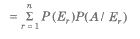
Let S be the sample space and let E₁, E₂,…., E_n be n mutually exclusive and exhaustive events associated with a random experiment. If A is any event which occurs with E₁ or E₂ or … or E_n then

P(A) = P(E₁)P(A / E₁) + P(E₂)P(A / E₂) + … + P(E_n) P(A / E_n)

Baye’s Theorem

Let S be the sample space and let E₁, E₂,…,E_n, be n mutually exclusive and exhaustive events associated With a random experiment. If A is any event which occurs with E₁ or E₂ or … or E_n then probability of occurrence of E_i, when A occurred,

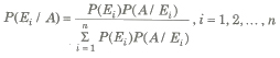
where, P (E_i), i = 1,2, , n are known as the priori probabilities

P (A / E_i), i = 1,2, , n are called the likelyhood probabilities

P (E_i / A), i = 1, 2, … ,n are called the posterior probabilities

Random Variable

Let U or S be a sample space associated with a given random experiment. A real valued function X defined on U or S, i:e.,

X : U → R is called a random variable.

There are two types of random variable.

(i) Discrete Random Variable – If the range of the real function X: U → R is a finite set or an infinite set of real numbers, it is called a discrete random variable.

(ii) Continuous Random Variable – If the range of X is an interval (a, b) of R, then X is called a continuous random variable. e.g., In tossing of two coins S = {HH, HT, TH , TT}, let X denotes number of heads in tossing of two coins, then

X (HH) = 2,X (TH) = 1, X (TT) = 0

Probability Distribution

If a random variable X takes values X₁, X₂,…., X_n with respective probabilities P₁, P₂,…., P_nthen

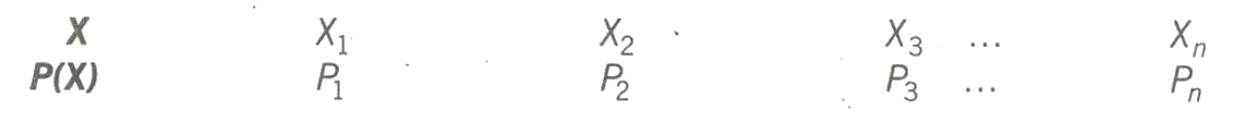
is known as the probability distribution of X.

or

Probability distribution gives the values of the random variable along with the corresponding probabilities.

Mathematical Expectation/Mean

If X is a discrete random variable which assume values X₁, X₂,…., X_n with respective probabilities P₁, P₂,…., P_n then the mean x of X is defined as

E(X) = X = P₁X₁ + P₂X₂ + … + P_nX_n = Σⁿ_{i = 1} P_iX_i

Important Results

(i) Variance V(X) = σ²_x = E(X²) – (E(X))²

where, E(X²) = Σⁿ_{i = 1} x²_iP(x_i)

(ii) Standard Deviation

√V(X) = σ_x = √E(X²) – (E(X))²

(iii) If Y = a X + b, then

(a) E(Y) = E(aX + b) = aE(X) + b

(b) σ²_y = a²V(Y) = a^2σ2_x

(c) σ_y = √V(Y) = |a|σ_x

(iv) If Z = aX² + bX + c, then

E(Z) = E(aX² + bX + c)

= aE(X²) + bE(X) + c

Binomial Distribution

Bernaulli Trial

In a random experiment, if there are any two events, “Success and Failure” and the sum of the probabilities of these two events is 1, then any outcome of such experiment is- known as a Bernaulli Trial.

Binomial Distribution

The probability of r successes in n independent Bernaulli Trials is denoted by P(X = r) and is given by

P(X = r) = ⁿC_rp^rq^{n – r},

where p = probability of success,

q = probability of failure

and p+q=l

Important Results

(i) If P = q, then probability of r successes in n trials is ⁿC_rpⁿ

(ii) If the total number of trials is n in any attempt and if there are N such attempts, then the total number of r successes is N(ⁿC_rp^rq^{n – r})

(iii) Mean = E(X) = x= np

(iv) Variance = σ²_x = npq

(v) Standard Deviation = σ²_x = √npq

(vi) Mean is always greater than variance

Poisson’s Distribution

It is the limiting case of binomial distribution under the following conditions

(i) Number of trials are very large, i.e., n → ∞

(ii) p → 0

(iii) np → λ, a finite quantity (λ A is called parameter)

The probability of r success for Poisson’s distribution is given by

P(X = r) = e ^{– λ}λ’ / r!, r = 0, 1, 2,…

For Poisson’s distribution

Mean = Variance = λ = np

Geometrical Probability

If the total number’ of outcomes of a trial in a random experiment is infinite, in such cases, the definitioin, of probability is modified and the
general expression for the probability P of occurrence of an event is given by

p = Measure of the specifie part of the region / Measure of the whole region

where, measure means length or al’~a or volume of the region, if we are dealing with one, two or three dimensional space respectively.

Application Based Result

(i) When two dice are thrown, the number of ways of getting a total r is

(a) (r – 1), if 2 ≤ r ≤ 7 and (b) (13 – r), if 8 ≤ r ≤ 12

(ii) Experiment with insertion of n letters in n addressed envelopes.

(a) Probability of inserting all the n letters in right envelopes

= 1 / n!

(b) Probability that all letters does not in right envelopes

1 – 1 / n!

(c) Probability of keeping al1 the letters in wrong envelope

1 / 2! – 1 / 3!+…+ (-1)ⁿ / n!

(d) Probability that exactly letters are in right envelopes

= 1 / r! [1 / 2! – 1 / 3!+ 1 / 4 -…+ (-1)^{n – r} / (n – r)!]

(iii) (a) Selection of shoes from a Cupboard Out of n pair of shoes, if k shoes are selected at random, the probability that there is no pair is

p = ⁿC_k2^k / ²ⁿC_k

(b) The probability that there is atleast one pair is (1- p).

(iv) Selection of Squares from the Chessboard – If r squares are selected from a chessboard, then probability that they lie on a diagonal is

4[⁷C_r + ⁶C_r +… + ¹C_r] + 2(⁸C_r) / ⁶⁴C_r

(v) If A and B are two finite sets and if a mapping is selected at random from the set of all mapping from A into B, then the probability that the mapping is

(a) a one-one function = ^n(B)P_n(A) / n(B)^n(A)

(b) a many-one function = 1 – ^n(B)P_n(A) / n(B)^n(A)

(c) a constant function = n(B) / n(B)^n(A)

(d) a one-one onto function = n(A)! / n(B)^n(A)